Cet article est également disponible en français.

The uncertainty calculation, even if not widely accepted by all industrialists, occupies more and more metrologists around the world. In order to help them out, the J.C.G.M. WG 1 published in 1995 the J.C.G.M. 100 document, better known as G.U.M. (Guide to the expression of Uncertainty in Measurement). This document is quoted for a long time in ISO standards. It is published by the AFNOR under its new reference NF ISO/CEI GUIDE 98-3 since July 2014.

The G.U.M. offers a probalistic approach of the measurement uncertainty. It essentially concerns random effects that impact on measurement results. Indeed in the spirit of the G.U.M., the systematic effects (which are not really enunciated) must be corrected, and nobody can throw this vision out. Actually it is one of the role of metrology, isn’t it?

Before going any further and questioning about the potential “pitfall” in the G.U.M., it is essential to remember what a random phenomenon is. For this purpose, the example of dice rolling is probably the most pedagogical.

When three dice are rolled, we cannot know the value of the faces sum that will appear since this sum is unreliable. Statisticians can only inform us about the likelihood that one value over another should appear. For example if we roll one die, the probability of making 1, 2, 3, 4, 5 or 6 is 1/6 (in case the dice are not loaded). Besides, statisticians have shown that under certain conditions frequently met, the likelihood of possible values occurring for a complex phenomenon (meaning it originates from effects of several elementary and random phenomena) follows a “normal distribution”. That normal distribution is defined by two parameters: its mean and its standard deviation. Thus, by knowing only two parameters it is possible to define the probability of any value produced by the random phenomenon.

Note: in metrology, that kind of random phenomenon (but not necessarily Gaussian) is typical. As an example, the climatic atmosphere in a measure environment: walking into a room, we do not know what the right temperature is but we can define the distribution, so the probability, of each practicable value.

Moreover, statisticians have shown that the variance of a complex random phenomenon is the sum of the elementary phenomenon variances that compose it (provided that elementary phenomena are individuals). The GUM is based on the additivity property of the variances. The evaluation of the measurement uncertainty of a process is based on the analysis of elementary phenomena, the evaluation of their respective variance (using experimental Type A or documentary Type B methods) to add them up. Obviously, the measurement model must be considered since it can introduce different sensitivity coefficients of 1 for each elementary phenomenon.

Thus, and to conclude on this reminder, a phenomenon is “random” when it varies, which means when we cannot predict the value that will come out during a given observation. The dispersion of such a random phenomenon is quantified by a mathematical concept called “standard deviation”. The square standards deviations of random elementary phenomena add up to give the global variance of the phenomenon of interest.

During the evaluation of the measurement uncertainty of a given process, it is quite usual to consider the calibration uncertainty as one of the uncertainty causes participating in the global uncertainty. It is therefore considered as one of the random elementary phenomenon altering the quality of the measure…

Yet the calibration uncertainty comes from the measurement imperfection during the calibration, which is a fact! It does not alter the reality of the calibrated object but only the knowledge we have of it! In the case of calibration masses for example, the masses are what they are and the mistake produced during the calibration does not change anything… So the calibration uncertainty is the expression of the operator imperfection, not the mass itself! If the calibration uncertainty has a random nature, the “real” value of the calibrated mass, in a given time, has nothing unreliable. It is what it is, even if we will never know what it really is!

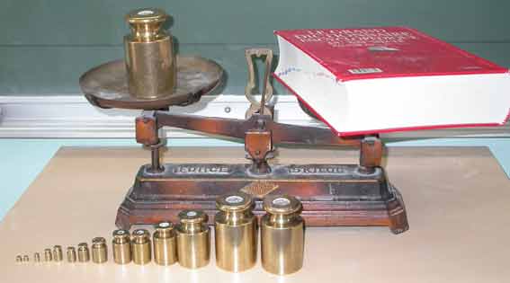
Let’s analyze together the above measurement process. The evaluation of the book mass requires calibration masses allowing the balance equilibrium. If the equilibrium is not perfect, the operator will have to read a deviation between the right pan and the left pan. That deviation will be added to the value of the equilibrium masses in order to determine the book mass. As the masses are not directly measured (only the weight of the objects is available), we need to take into account the differences of buoyancy between calibration masses (density MV1) and the book (density MV2). Buoyancy equals, in these two cases, the weight (Mass x acceleration “g”) of the volume of the displaced fluid (here of the air). We need also to take into account the temperature, the pressure and the relative humidity. I still don’t see how the calibration uncertainty participates to this measurement process… I obviously understand this uncertainty, indicated during the calibration of masses, does not let me know the real value of those masses. However, the mistake produced during the calibration does not occur during the measure of my book… My masses are what they are, I do not know their real value but they have nothing random (their weight can vary depending on the measurement conditions, but their mass do not). To add a random effect (the calibration uncertainty) in the report of uncertainty causes concerning my book measurement has no statistical sense! It is a kind of tip of which relevance is questionable because the sum of the variances makes only sense for the random phenomenon…

In this case, the probalistic approach shows its limits. If it undeniably excels in quantifying the random phenomenon, it does not take into account the systematic effects of which we do not know the real value (inside the interval). It is the case here, just as in many other situations. Since we mention the masses, we can also mention the question of the value of the acceleration local coefficient, noted traditionally “g”. In a given place, it is systematic. We measure it, we inexorably meet an uncertainty. Nevertheless, in a measurement process of strength (or of mass) in a given place, the “g” value is not “probabilistic”. Again, it is what it is, only its reality is not available to us! It is very different considering this lack of knowledge from the probabilistic angle (as it is the case nowadays) that from the real angle: a deterministic (systematic) value, but unknown. This is indeed the case for “g”, such as for the real value of the calibration masses, but also such as numerous cases in metrology. The calibration uncertainty does not contribute directly (under its random form clearly – during the calibration we can hope the laboratory corrects the systematic effects in a smart way) in the report of the process uncertainty causes. However, it leads to a doubt about the real value of a quantity (mass, “g” or other). That doubt can be materialized by an interval in which we can determine the eventual quantity of interest (mass, value of local “g”, or else)…

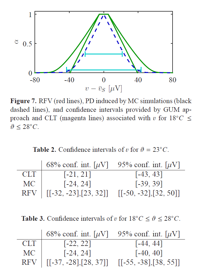
If the “probabilistic” approach does not resolve that question, the “possibilistic” approach seems to bring a solution to this frequent situation in metrology. The “possibilistic” approach calls on the concept of the “blurred variables”. In this world, calculation strategies have been developed to “add up” (read “associate”) intervals of “possibilities”; whereas the probabilistic world sums variations. The objective of this first article on this topic is not the description of the “possibilistic” strategies. Here the concern is, in a first instance, to warn metrologists on this question that will deserve to be developed in the future, from my point of view.

A particularly dynamic Italian team, carried out by Alessandro Ferrero and Simona Salicone from the Polytechnic School of Milan, regularly publishes about this fascinating approach of possibility. I will have the honour to give a lecture with them about that topic during the next international congress of metrology in September 2015 in Paris. Until that time, I will come back to you to tell you more about that theme…

Nevertheless, I cannot resist the pleasure of showing you a “classical” illustration of the “possibilist” world, so you will start to get used to it…